This article is an automatically translated version of the original Japanese article. Please refer to the Japanese version for the most accurate information.

This is sustainacraft Inc.'s 6th Newsletter.

In our third newsletter, we introduced the issue of junk Carbon Credits, one of the causes of which was the difficulty in setting a Baseline. The Baseline refers to the counterfactual trend of deforestation – "what if no forest conservation project had been undertaken?" – but current Credit calculation Methodologies do not always adequately consider such counterfactual settings. On the other hand, estimation methods that do account for such settings have a rich body of research in the field of Causal Inference, and it is expected that this knowledge will be applied to Methodologies in the future.

Therefore, this time, with Baseline estimation in forest projects in mind, we will introduce current major Credit Methodologies and two Causal Inference methods, comparing their characteristics. This newsletter will be somewhat more technical than previous ones, but we hope it will be a useful reference for organizing the problems with current Methodologies, alternative approaches, and the differences between them.

PickUp Section

Baseline Setting Methods in VM0007

(Source: VM0007 REDD+ Methodology Framework (REDD+MF), v1.6)

• One of the most common Methodologies for measuring the effectiveness of REDD+ projects for forest conservation is Verra's VM0007.

• In VM0007, to calculate the Baseline for the Project Area (hereafter PA), an area called RRD (Reference Region for projecting rate of Deforestation) is established and treated as a control group.

  • The RRD is selected to be as similar as possible to the PA in terms of land, economic, and social environment, referencing the following factors:

    • deforestation agents (e.g., illegal agricultural conversion by small-scale farmers)

    • forest type, soil, elevation, slope

    • infrastructure development such as roads, rivers, and settlements

    • other social conditions: policies, regulations, ethnic composition of land, presence of gangs, etc.

  • As an example, the figure shows the PA (green) and RRD (yellow) actually set for the Valparaiso project carried out in Acre state, Brazil (Source: Project PDD).

    

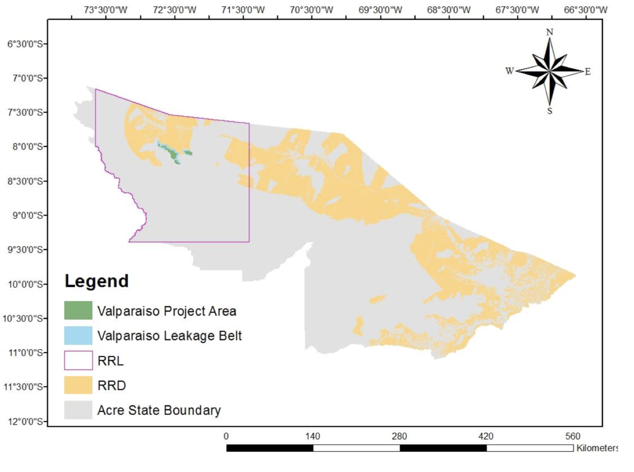
• The Baseline for the PA is calculated using the RRD's past average deforestation rate.

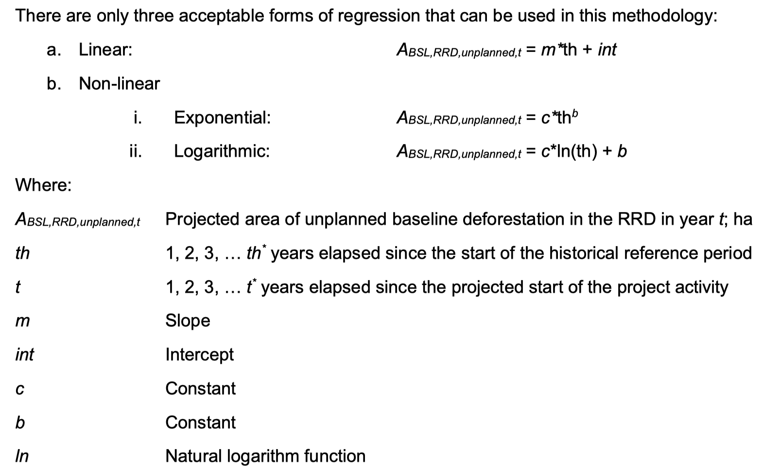
  • Using data from the past 10-12 years before project commencement, one of the following is adopted: 1) linear model, 2) nonlinear model, or 3) simple historical average.

  • First, the use of a model is considered, and functional forms are specified for both linear and nonlinear models (nonlinear models cannot be used if data is available for fewer than 5 time points).

  

  • When using a model, special attention must be paid to the following:

    • The model is statistically significant at a 5% significance level.

    • R2 is 0.75 or greater.

    • There is no bias.

  • If these conditions are not met, the simple historical average is used as the Baseline.

• Below is an example of the Baseline set for the Valparaiso project. Our verification results, based on the PDD and using open forest data, are also provided.

  • Legend

    • Yellow (solid line): Deforestation rate in RRD as stated in the PDD

    • Blue (solid line): Deforestation rate in RRD set by us based on the PDD

    • Red (solid line): Deforestation rate in PA calculated by us

  • In this example, neither the linear nor the nonlinear model meets the accuracy requirements above, so the simple historical average is adopted.

  • Therefore, the yellow/blue horizontal dotted line serves as the Baseline, and Credits are Issued based on the difference from the red line1.

  

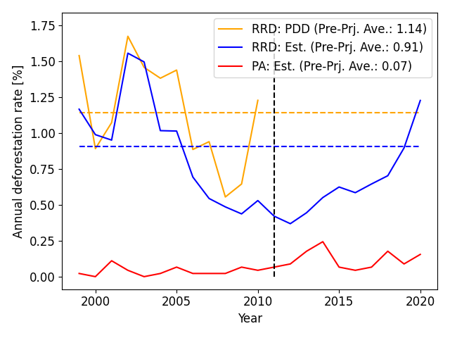
  • The reported values from the project and our verified values do not perfectly match due to differences in RRD locations and forest data used.

  • Nevertheless, compared to the actual deforestation rate in the PA, the Baseline appears to be set excessively high.

• As in this example, in VM0007, depending on the selection of the RRD, the Baseline can be set excessively high compared to the levels prior to project commencement.

• Furthermore, changes in external factors that occur after project commencement cannot be reflected in the Baseline.

• A useful method for addressing these issues, as introduced in our third newsletter, is the Synthetic Control Method.

Baseline Estimation Methods Using SCM

(Source: Abadie et al., 2010)

• In the Synthetic Control Method (SCM), to eliminate the arbitrariness in selecting the RRD, a hypothetical PA time series is constructed by appropriately weighting the time series within the RRD2.

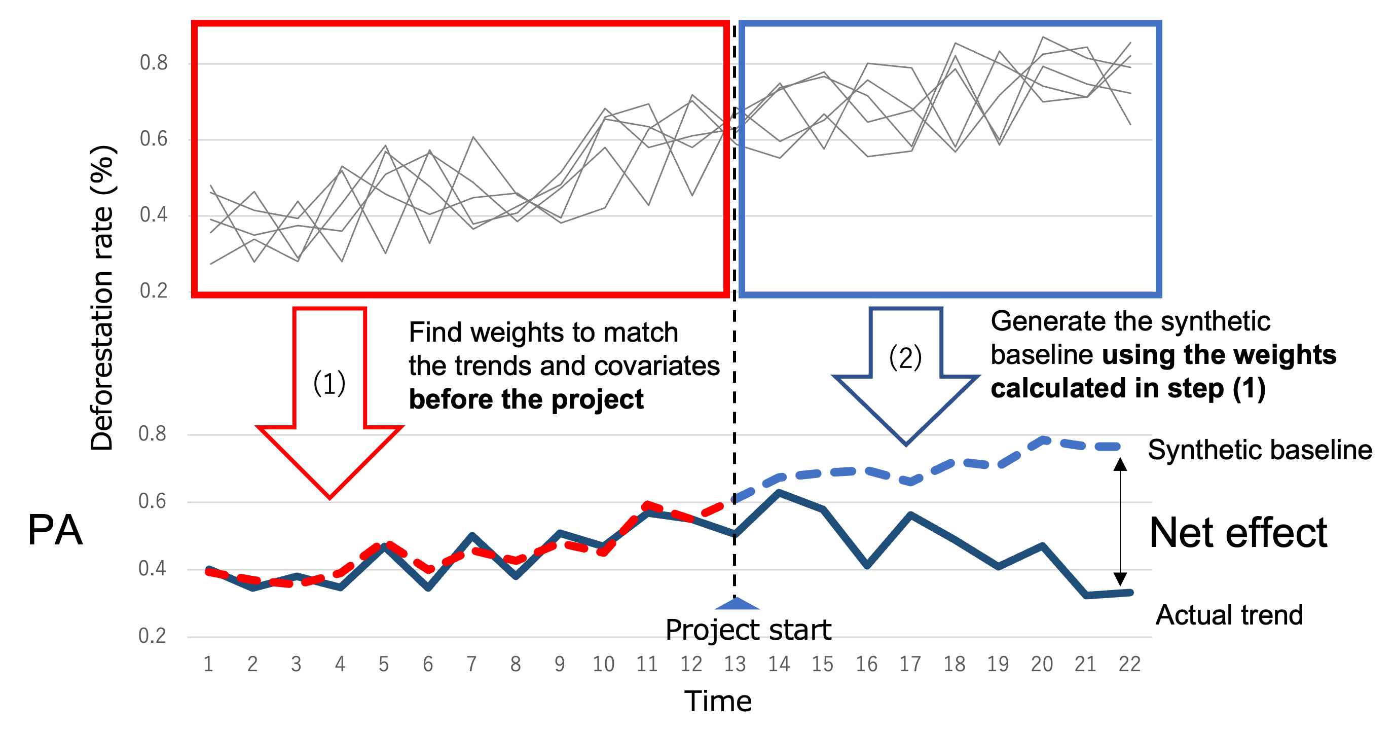
• The estimation steps for SCM are briefly illustrated below.

  • Weights are determined such that the linear combination of time series in the RRD, up to the project commencement, closely approximates the PA's time series.

  • Estimation aims to make not only the deforestation rate time series but also the vector including covariates similar. This adjusts for confounding factors, enabling appropriate comparison.

  • Using the derived weights, the PA's Baseline is estimated as a linear combination of the RRD's time series after project commencement.

  

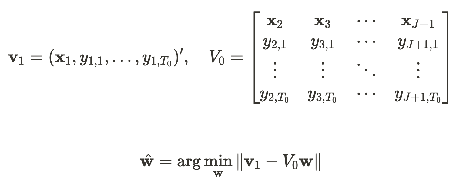
• Expressed in mathematical formulas, it is as follows:

  • x_j is a vector summarizing covariates in area j, y_{j,t} is the deforestation rate in area j at time t, w is a vector summarizing the weights applied to each location, and T_0 is the project commencement time.

  

  • The project effect at time t (>T0) is estimated using the derived weights as follows:

  

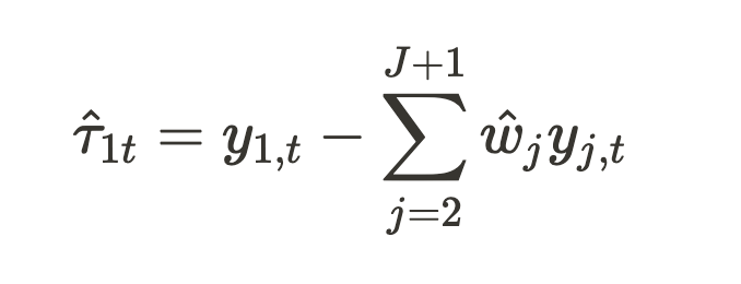
  • Abadie et al. (2010) also demonstrate that, under appropriate conditions, the Baseline estimated this way is unbiased (i.e., unbiased estimation is possible in expectation).

• The strengths of SCM include the following points:

  • Covariates are adjusted, allowing for proper isolation of the project's effect.

  • The Baseline is estimated to change continuously from actual values before and after project commencement (in VM0007, as in the Valparaiso example, the Baseline may deviate significantly from actual values prior to the project).

  • The impact of external factors other than the project (if they also affect the RRD) is reflected in the Baseline.

  • Weights are automatically set, which can reduce the arbitrariness in selecting the RRD.

• On the other hand, the weaknesses include the following points:

  • Since calculations use actual values, it cannot predict the Baseline before project commencement and can only be used for ex-post evaluation.

• As introduced in our third newsletter, SCM's strengths are attractive in addressing criticisms of junk Carbon Credits.

• However, when considering the formation of new projects or investments, the aspect of forecasting—"how many Credits might the project generate in the future?"—is crucial, but SCM makes predictions before project commencement difficult.

• As one model considered useful for this point, we will finally introduce a method using Bayesian structural time-series models.

Baseline Estimation Methods Using Bayesian Structural Time-Series Models

(Source: Brodersen et al., 2015)

• The method using Bayesian Structural Time-Series Models (BSTS) was proposed by Brodersen et al.'s team at Google.

  • It is also a well-known model implemented as the {CausalImpact} package in R. Hereafter, for simplicity, it will be referred to as the BSTS model3.

• The basic idea is similar to SCM. By focusing on the time series prior to project commencement, a model is trained to explain the PA's time series using multiple time series within the RRD, and then applied to the RRD's time series after project commencement to estimate the PA's Baseline.

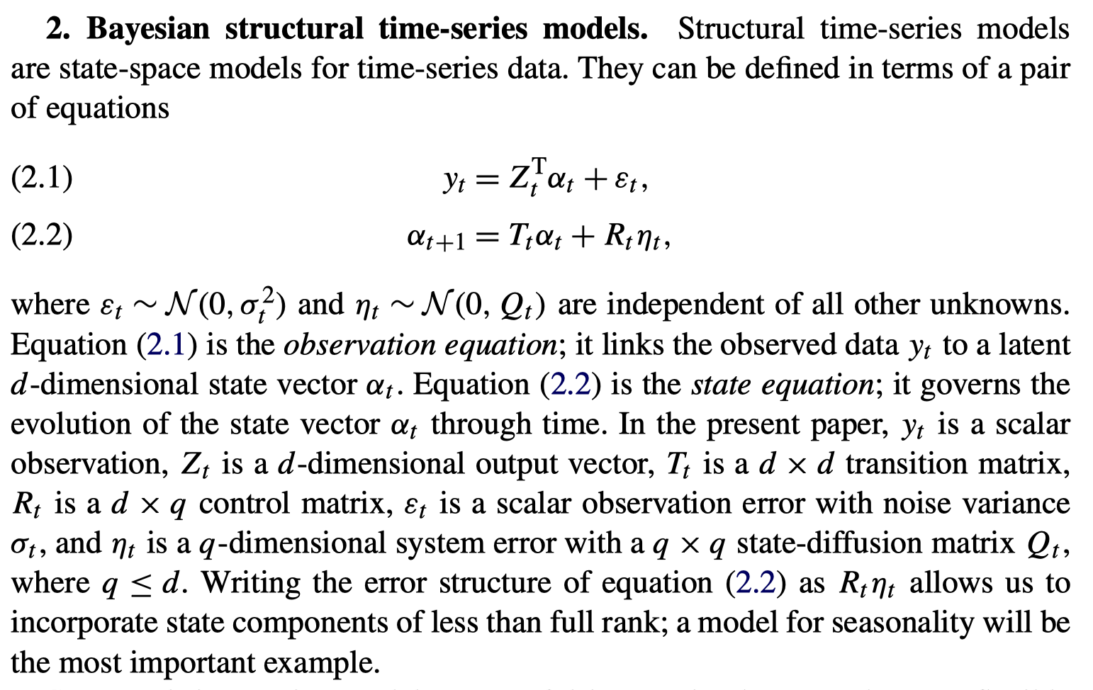
• What differs from SCM is the use of a state-space model for the PA's time series and the relational equation connecting it with the RRD's time series.

• The mathematical expression is as follows:

  • In the context of Baseline setting, y_t is the deforestation rate in the PA, Z_t is a vector summarizing multiple deforestation rates in the RRD, and α_t is the weight vector.

  • Parameters are estimated by training with data up to project commencement, and then applied to the RRD's time series (Z_t) after project commencement to obtain the estimated PA Baseline.

  

• The strengths of BSTS include the following points:

  • It can predict the Baseline after project commencement, at the stage prior to project commencement.

    • While the original paper models the variable corresponding to SCM's weights (α_t), it is believed that by reformulating this not as weights but as a model for the RRD's time series (Z_t), predictions can be made prior to project commencement.

    • While it would be a simple time series prediction before project commencement, if the RRD's time series becomes available after project commencement, evaluation using conditional expectation becomes possible, allowing for a unified framework for prediction and ex-post evaluation.

  • The uncertainty of the estimated values can be easily assessed using Bayesian posterior distributions.

  • By placing a Spike-and-Slab prior, variables with high explanatory power can be automatically selected from numerous time series in the RRD.

• On the other hand, the following points can be considered weaknesses:

  • Since the covariate adjustment mechanism is not explicitly included, appropriate estimation may not be possible without some adjustment at the RRD selection stage.

  • Since it directly models the relationship between PA and RRD based on time series prior to project commencement, it is difficult to reflect the impact of external factors that occur after commencement.

Comparison of Methods

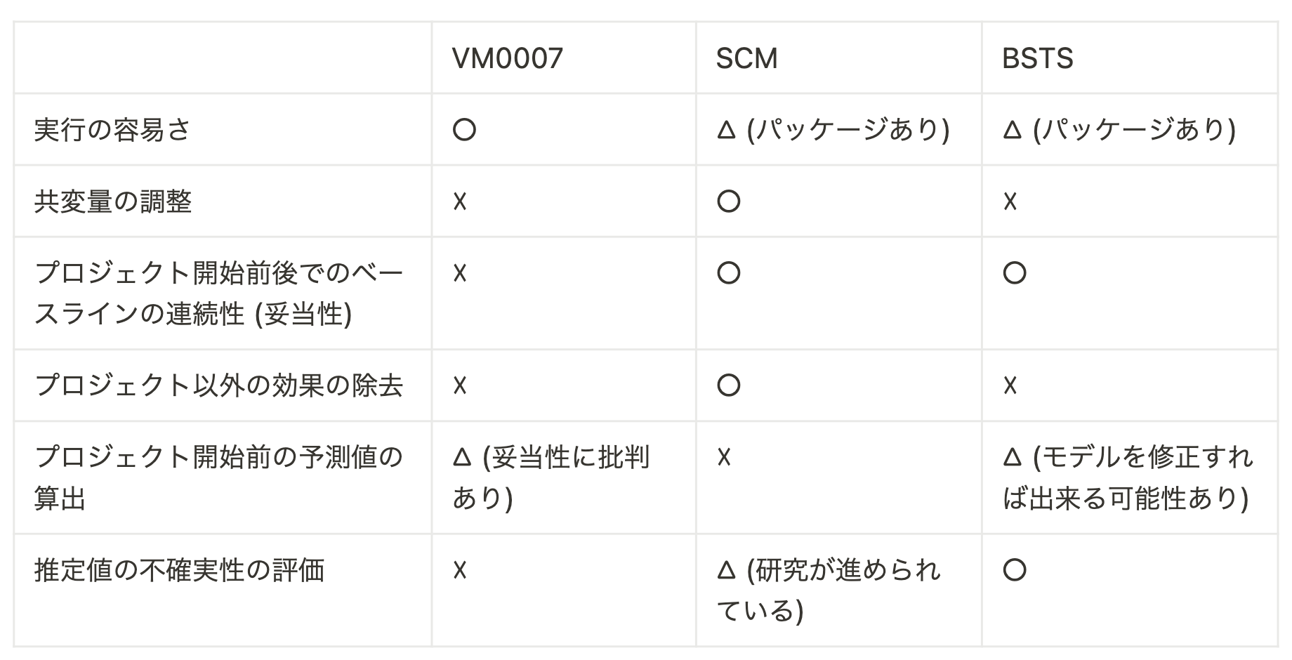
• The characteristics of the three methods introduced this time are summarized in the table below.

• While neither of the two Causal Inference methods introduced is inherently superior, it is clear that each can partially address the issues of existing Methodologies.

  

• Furthermore, the common approach among these methods of "taking the difference between two time series to determine causal effect" can be understood as an extension of the Difference-In-Differences (DID) method, frequently used in policy impact research.
• However, for DID estimators to have statistical validity, several assumptions are required, one of which is the parallel trends assumption. In this context, it implies that "the effect of implementing a project does not differ between the PA and the RRD."
• However, even if similar regions are selected, if land, environmental, and economic factors differ between the PA and the RRD, the project's effects will naturally also differ, making it highly probable that this assumption is not met.
• While SCM mitigates this assumption by calculating weights that account for covariate adjustment, VM0007 and BSTS do not sufficiently incorporate this, meaning the difference between the project's actual outcome and the estimated Baseline may not be an appropriate estimate.
• Thus, for appropriate impact verification, it is crucial to carefully confirm whether confounding factors other than the project have been adjusted for. Causal Inference methods provide one systematic framework for addressing such issues and are likely to offer important insights for developing Carbon Credit Methodologies.

News from sustainacraft

• Participated in VivaTechnology Paris 2022 (2022/06/15-17)

  • On 06/15, we exhibited at the booth of French telecommunications company Orange, and on 06/16-17, at the JETRO Japan Pavilion booth.

• Implementation of Third-Party Allotment of Shares

  • Implemented a third-party allotment of shares, with Mitsubishi UFJ Innovation Partners No. 2 Investment Limited Partnership, a fund of Mitsubishi UFJ Financial Group, as the subscriber.

  • References: Our release, MUIP's press release

• Featured in the Nikkei Shimbun Digital Edition and Nikkei Shimbun print edition (July 6).

  • Digital edition title: Sustainacraft to enter Carbon Offset Verification Business.

  • Print edition title: Offsetting CO2 Emissions, Verifying Implementation.

Closing remarks

In this newsletter, we introduced Methodologies and estimation methods in a general form. However, in actual projects, the background of deforestation, environmental conditions, and policies differ, so a naive application of these methods is often insufficient. It is crucial to understand the specific characteristics of each project and meticulously deconstruct its elements.

How REDD+ projects are designed and what their outcomes have been are publicly available in the form of PDDs and Validation reports, accessible to anyone. These are very useful for envisioning actual project operations and understanding project-specific characteristics, so we encourage anyone interested to take a look.

This concludes sustainacraft's Newsletter #6. In this newsletter, we plan to disseminate information in Japanese on NbS approximately bi-weekly to once a month.

Our company profile can be found here for your reference.

Disclaimers:
This newsletter is not financial advice. So do your own research and due diligence.